Sigmoid Neuron

This article covers the content discussed in the Sigmoid Neuron module of the Deep Learning course and all the images are taken from the same module.

In this article, we discuss the 6 jars of the Machine Learning with respect to the Sigmoid Model but before beginning with that let’s see the drawback of the Perceptron Model.

Sigmoid Model and a drawback of the Perceptron Model:

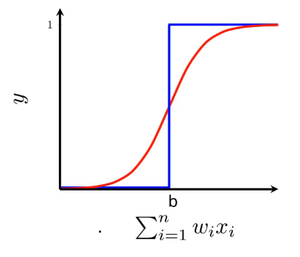
The limitation of the perceptron model is that we have this harsh function(boundary) separating the classes on two sides as depicted below

And we would like to have a smoother transition curve which is closer to the way humans make decisions in the sense that something is not drastically changed, it slowly changes over a range of values. So, we would like to have something like the S-shaped function(in red in the below image).

And we have the Sigmoid family of functions in Deep Learning of which many of the functions are S-shaped. One such function is the logistic function(it is one smooth continuous function) and this function is defined by the below equation:

So, we will now approximate the relationship between the input x(which could be n-dimensional) and the output y using this Logistic function(Sigmoid function). This function would have some parameters and we would try to learn the parameters using the data in such a way that the loss is minimized.

Now to visualize this function, we can take some values of x and y and plot it to see what it looks like, for example in the below case, we are plotting (‘wx + b’) on the x-axis and ‘y’ value on the y-axis.

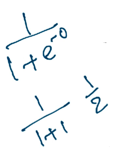
If ‘wx + b’ is 0, then the equation(y) is reduced to:

Let’s try some other value: