Optimization Algorithms: Part 1
This article covers the content discussed in the Optimization Algorithms module of the Deep Learning course and all the images are taken from the same module.
Limitation of Gradient Descent:
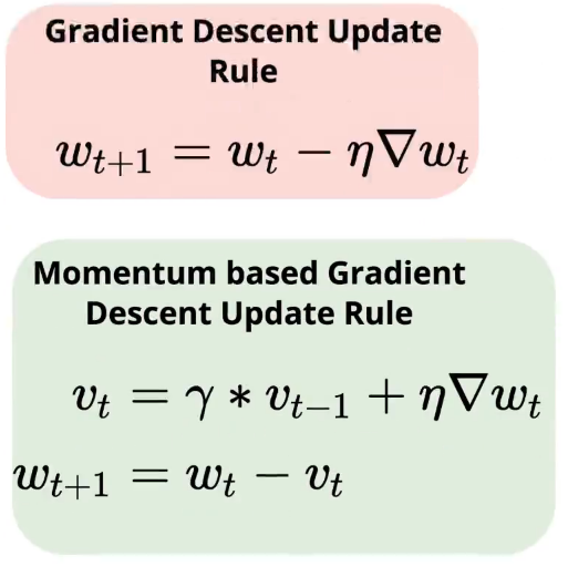
We have seen the Gradient Descent update rule so far and even when we are doing backpropagation, at the core of it is this update rule where we take a weight and update its value based on the partial derivative of the loss function with respect to this weight:

The question that we look at now is that How do we compute this gradient or in other words, what data to use when computing this gradient: should we use the entire data or should we use a small part of the data or should we use one data point. This decision will result in Batch Gradient Descent, Mini Batch Gradient Descent or Stochastic Gradient Descent.

The other question we look at is: once we have computed the gradients, how to use it, meaning how to use the gradient when updating the parameter value. Instead of just subtracting the gradient value, shall we look at all the past gradients and the current gradient and then take a decision based on that or shall we just take into consideration only the current gradient value?

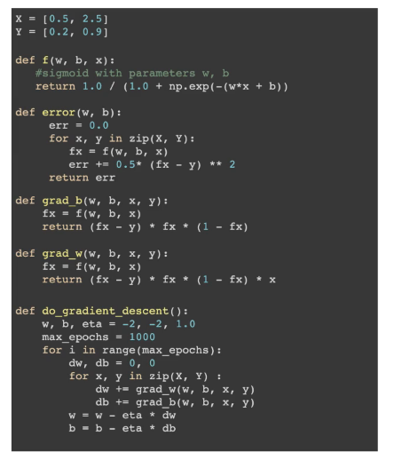
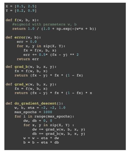
The code for the Gradient Descent is:

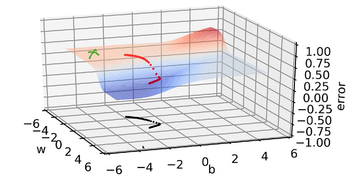
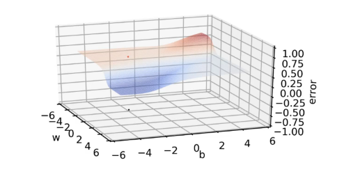
We have randomly initialized the parameters w, b(blue point in the below image represent the parameters w, b):

The red dot in the above image is the loss value corresponding to this particular value of w, b(which is randomly initialized).
Now we will run the gradient descent algorithm and see how the loss value changes:
After a few iterations, the situation is like the below:

From above, we can say that in every successive iteration/epoch, w and b are changing very little and when we are moving from one value of w, b to another value of w, b, they are almost connected to each other, we are not taking larger steps. So, in this flat region, the values are changing very slowly and when we come at the slope region(in the valley), w and b values are changing very drastically
And again as we enter the flat region, we can see very small changes in w, b values.

At the top red portion(light red portion) where we started off with this algorithm, the loss surface had a very gentle slope, it was almost flat and once we are entering this blue region(there is a valley at the bottom), so there was a sudden slope, the slope was very high and at that point, we are seeing larger changes in w, b and again once we reach the bottom portion, that portion is again flat, there also the values are not getting updated very fast, the moment is very slow and two successive values of w, b are very close to each other.
So, in the gentle areas, the moment is very slow and in the steep areas, the moment is good.
A deeper look into the limitation of Gradient Descent:
Let’s take a function and we will see what does the slope of the function means and how it is related to derivative and how does it explain the behavior(in certain regions the moment was steep and in certain regions the moment was fast) that we discussed above
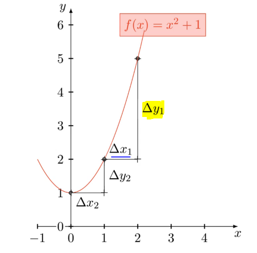
The derivative at any point is the change in the y value(in yellow in the above image) divided by the change in the x value(blue underlined in the above image). So, it tells how does the ‘y’ changes when ‘x’ changes.
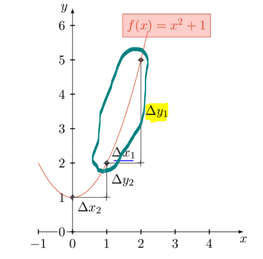
In the region(in elliptical boundary in above image), the slope is very steep, if we put a ball at the upper point, it will come down very fast, here for a change of value of 1 in x, the value of y is changing by 3, the derivative is larger whereas in the elliptical region in the below image, the slope is gentle.
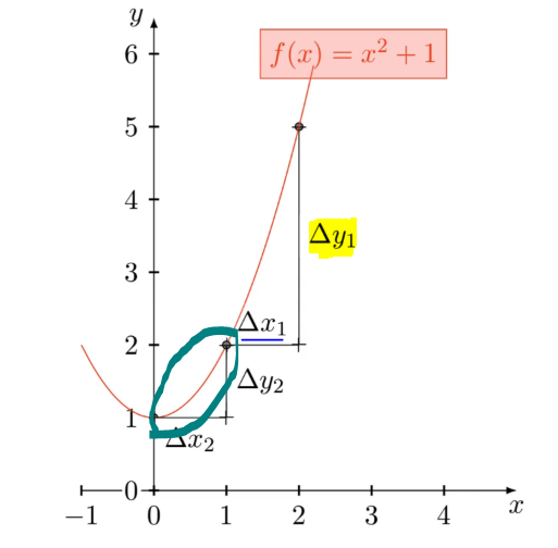
and a change of 1 in the x corresponds to a change of 1 in y, so the derivative is smaller as compared to the above region where the slope is steep.
So, we see that if the slope is very steep the derivative is high and if the slope is gentle the derivative is small.
The value of the parameters are changing in the proportion of the derivatives so, in the regions where the derivative is small, ‘w’ is also going to change by a small quantity and in the regions where the derivative is large, the parameters are going to change by a large quantity.
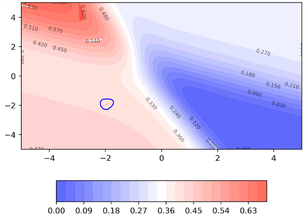
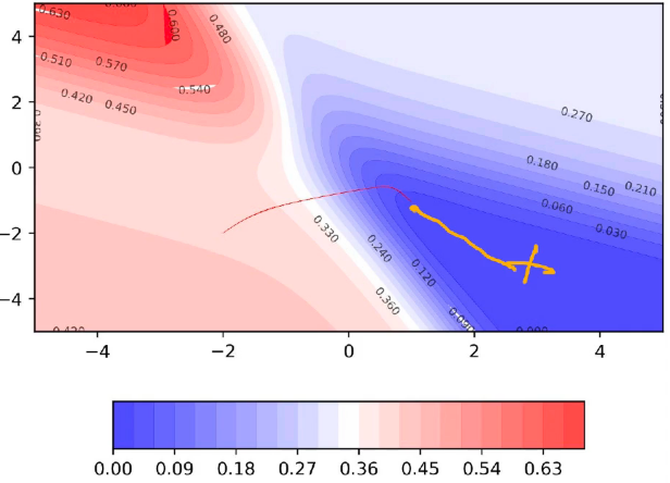
Now taking the above scenario, let’s consider when the random initialization corresponds to the green marked point in the below image:
The entire region is flat from the initialization point up to(underlined in pink in below image) the start of the red line, so it will take a lot of time to travel up to this red point i.e the start of the valley and then once it goes into the valley, it will start moving faster.
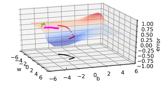
It might take 100–200 epochs just to reach the edge of the valley and then jump into the valley and that’s not acceptable as we have to run many epochs just to make a small change in the loss value which is not a favorable situation.
We should try to change gradient descent in a way so that on the gentle slope surfaces, the moment becomes faster.
This bothers us as we are initializing the parameters randomly and if so happens that we have initialized these parameters at a place where the surface is very flat, then we need to have many many epochs just to come out of that flat surface and enter into a slightly steep region and from there on we can see slight improvement in the loss function.
Introducing Contour Maps:
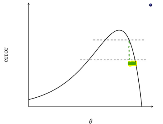
If we see the loss/error surface for the above case from the front and plot it in 2D, we will get:
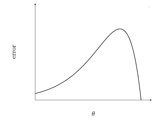
If we make two horizontal slices on this surface, each horizontal slice would result in a plane cutting through the 3D surface and wherever the plane is intersecting with the 3D surface or the portion it is cutting through, around that entire perimeter on the 3D surface, the loss function/value is the same.
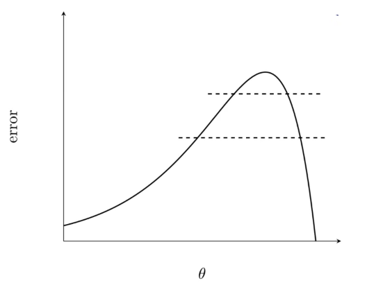
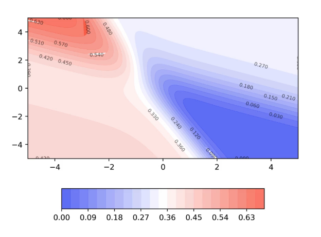
Now after making these 2 slices, if we look at it from the top, it would appear to be:
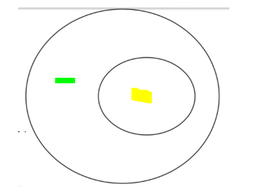
The ellipse with yellow in it would correspond to the first slice and the other ellipse with green in it would correspond to the second slice through the surface.
The loss value is the same at the entire boundary of the ellipse. So, the first point of reading contour maps is that whenever we see a boundary that means the entire boundary has the same value for the loss function.
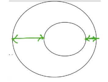
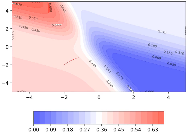
Now we have shown the distance between the two ellipsed from two ends. One of the distance is small compared to the other one. Reason for this is that the portion circled in the below image
corresponds to the difference in the green in the below image and there the surface is very steep.
So, whenever the slope is very steep between two contours, then the distance between the two contours would be small.
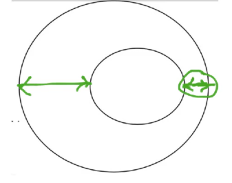
Similarly the region in blue in the below image

corresponds to the difference in blue in the below image:
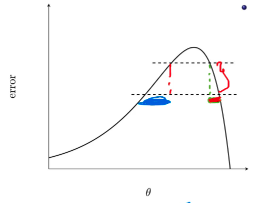
and the slope was a bit gentle here as compared to the red slope and therefore, whenever the slope is gentle when going from one contour to the other contour, then the distance between two contours is going to be high.
- A small distance between contours indicates a steep slope along that direction.
- A large distance between contours indicates a gentle slope along that direction.
Visualizing Gradient Descent on a 2D Contour Map:
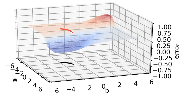
We have the 3D surface as:
And the same in 2D looks like:
The moment of the loss values on this 2D would look like as:
Since we started off in the flat region, the values would move very slowly along this region.
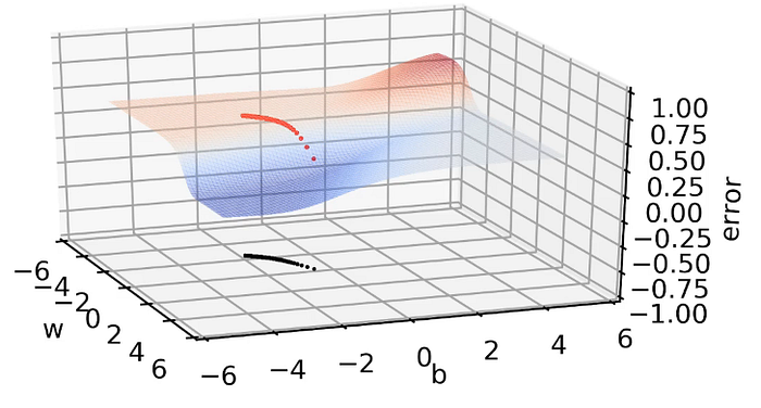
Now it has reached the edge of the valley where the slope is steep, we can see larger moments:
Momentum Based Gradient Descent:
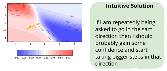
If the gradients are continuously pointing in the same direction, then it would be good if we take large steps(update) in that direction.
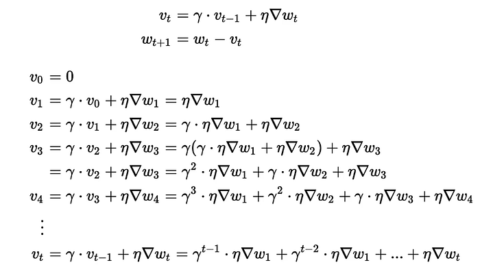
It’s like taking an average of all the gradients that we have computed so far instead of just relying on the current gradient and the average does not give equal weightage to all the gradients, it’s exponentially decaying weightage to all the previous gradients.
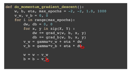
Code for Momentum Based GD:
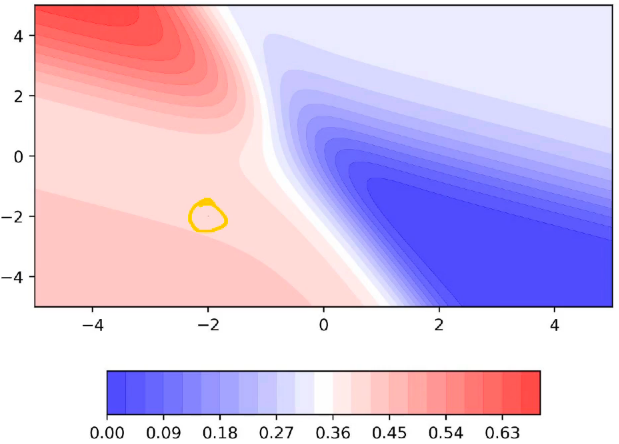
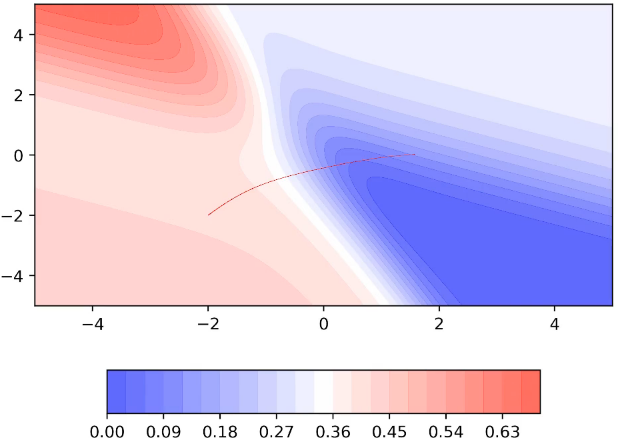
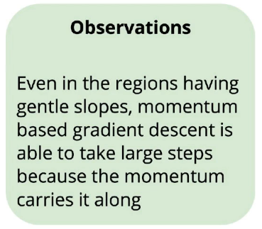
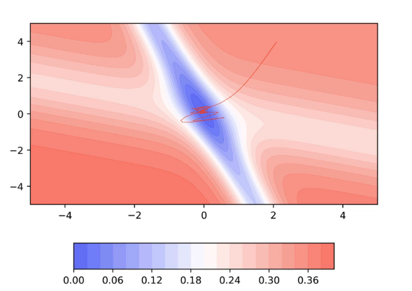
Visualizing Momentum Based GD:


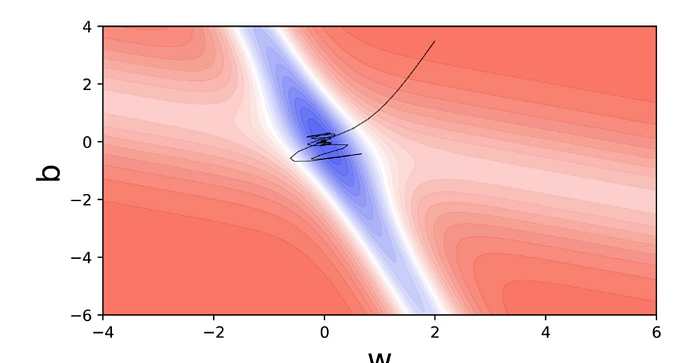
A disadvantage of Momentum based GD:
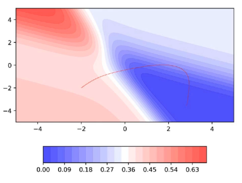

Let’s plot the 2D error surface for another scenario:
The intuition behind Nesterov Accelerated Gradient Descent:
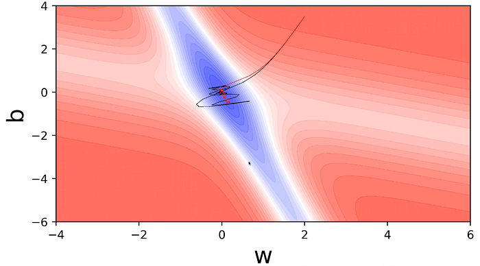
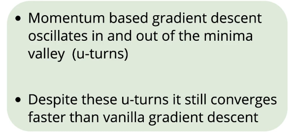
We want an algorithm that converges faster than Vanilla GD but does not makes a lot of u-turns as Momentum GD. So, we discuss Nesterov Accelerated Gradient Descent in which the no. of oscillations(u-turns) are reduced compared to Momentum based GD.
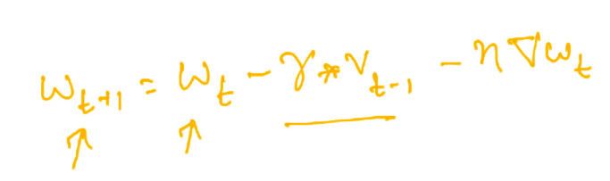
In Momentum GD, the update would look like:
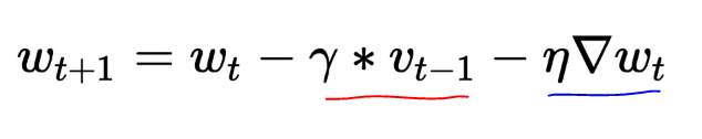
In the above equation, we have one term for history(underlined in red) and one term for the current gradient(underlined in blue).
We know that in any case, we need to move by the history component, then why not move by that much first and then compute the derivative at that point and we should then move in the direction of that gradient.
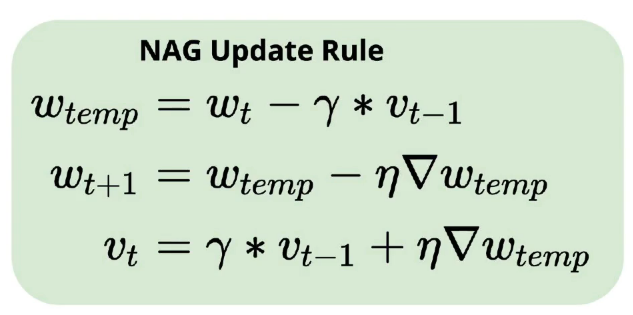
Code for NAG:

In case of Momentum GD, we have:
To start with, both Momentum GD and NAG would have the same curve/line and only in the valley having a steep slope, we would see the effect of NAG as it would take shorter u-turns.